Kalman Filter RLC

The RLC circuit above can be expressed by the following equation
The equation can be expressed as two first order differential equations using the following method.
$$ x_{1} = I_{L} $$
$$ x_{2} = \dot{I}_{L}$$
and
Replacing variables with state variables $\bf{X}$
$$ \frac{x_{1_{k+1}} - x_{1_{k}}} {\Delta t} = x_{2_{k}}$$
rearranging gives the future value for $x_{1}$
$$ x_{1_{k+1}} = \Delta t x_{2_{k}} + x_{1_{k}} $$
The same method is then applied to $x_{2}$
$$ \frac{x_{2_{k+1}}- x_{2_k}}{\Delta t} = -\frac{x_{1_k}} {LC} -\frac{x_{2_{k}}}{RC} + \frac{I_k}{LC} $$
Giving the future value for $x_{2}$
$$ x_{2_{k+1}} = -\frac{\Delta t x_{1_k}} {LC} - x_{2_{k}}\left (1- \frac{\Delta t}{RC} \right) + \frac{\Delta t I_k}{LC} $$
The two equations can now be expressed in state space formalism. I have shifted the time step by -1 so $x_{1_{k+1}} $ is now $x_{1_{k}}$. This is done to maintain accordance with the kalman filter framework as shown below by the state transition model.
where
- $\hat{\bf{X}}$ - estimated state
- $\bf{X_{k-1}}$ - previous time steps estimated true state (combination of estimate and measurement)
- $\bf{F}$ - state transition model
- $\bf{B}$ - control input model
- $\bf{U}$ - control input
From here on, a hat above a variable indicates a predicted state and a tilde is a measured variable.
The voltage induced across an inductor is equal to the rate of change of current passing through it multiplied by its inductance.
The correction matrix takes the predicted value and adjusts it based on a measurement. How much the measurement is incorporated into the prediction is dependent on the Kalman gain.
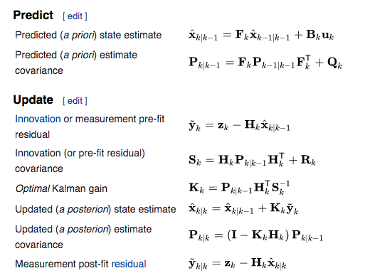
This is all that is needed in terms of design. The rest of the algorithm follows the formula below taken from Wikipedia.
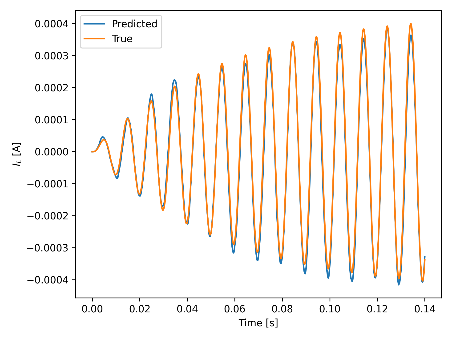
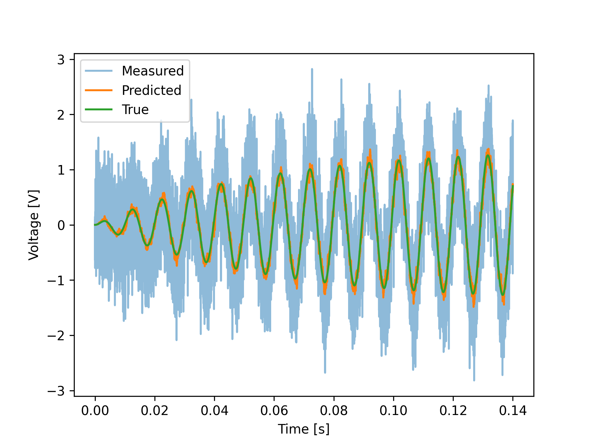
Results

Python Implementation
The implementation is made in a jupyter notebook which can be downloaded here. For ease of viewing I have pasted the code segments here -
Kalman RLC NotebookRequirements
%matplotlib qt
import numpy as np
import matplotlib.pyplot as plt
from numpy.linalg import inv
import copy
Transition Model
def prediction(Il,Ildot,I,t):

    L = 5
    C = 500e-9
    R = 50e3

    A = np.array([[1, t],
                  [-t/(L*C), 1 - (t/(R*C))]])

    X = np.array([[Il],
                 [Ildot]])

    B = np.array([[0],
                  [t/(L*C)]])

    U = I

    X_prediction = A.dot(X) + B.dot(U)


    return X_prediction
#time
T = 0.14
t = np.linspace(0,T,100e3*T)

#initialise inductor current and its derivertive
Il_true = np.zeros(len(t))
Ildot_true = np.zeros(len(t))

#cicuit component definitions
L = 5
C = 500e-9
R = 50e3
#create input signal
wr = 1/np.sqrt(L*C)

I_true = 25e-6 * np.sin(wr * t)

#time step
dt = t[1] - t[0]

#create True data
I = np.zeros((2,len(t)))

for i in range(1,len(t)):
    a =  prediction(I[0][i-1],I[1][i-1],I_true[i-1],dt).T
    I[:,i] = a

Il_true = I[0]
Ildot_true = I[1]

V_true = L*Ildot_true
noise = np.random.normal(loc=0, scale=0.5, size=len(t))
V_meas = V_true + noise
#state transition model
A = np.array([[1, dt],
              [-dt/(L*C), (1 - (dt/(R*C)))]],dtype='float')

#process noise(model noise)
Q = np.array([[4e-9, 0],
              [0, 4e-9]])

#measurement noise
R = np.array([[4]])

#Initial Predicted (a priori) estimate
P=Q
#store values for plotting
Il_a = np.zeros([len(t)])
Ildot_a = np.zeros([len(t)])

#initial values
Il_a[0]    = 0
Ildot_a[0] = 0

#set the input matrix to be the true input
I_a = I_true

# for i in range(1,len(t)):
for i in range(len(t)):
    #prediction
    X_hat = prediction(Il_a[i-1], Ildot_a[i-1], I_a[i-1],dt)

    #predicted estimate covariance
    P_hat = np.diag(np.diag(A.dot(P).dot(A.T))) + Q

    #observation matrix v(t) = Ldi/dt
    H = np.array([[0,L]])

    #innovation covariance
    S = H.dot(P_hat).dot(H.T) + R

    # Kalman Gain
    K = P_hat.dot(H.T).dot(inv(S))

    #measurement - prediction
    y = V_meas[i] - H.dot(X_hat)

    #updated state estimate
    X = X_hat + K.dot(y)

    #Updated (a posteriori) estimate covariance
    P = (np.identity(2) - K.dot(H)).dot(P_hat)

    #update values
    Il_a[i]    = X[0]
    Ildot_a[i] = X[1]